Rough Volatility

Bergomi's model revisited

Variance swap

A variance swap with maturity $\mathrm{T}$ is a contract which pays out the realized variance of the logarithmic total returns up to $\mathrm{T}$ less a strike called the variance swap rate $V_0^T$, determined in such a way that the contract has zero value today.

The annualized realized variance of a stock price process $\mathrm{S}$ for the period $[0,T]$ with business days $0=t_0<\dots <t_n=T$ is usually defined as $$R{V}^{0,T}:=\frac{d}{n}\sum _{i=1}^n{\left(\log \frac{S_{t_i}}{S_{t_{i-1}}}\right)}^2$$ The constant $d$ denotes the number of trading days per year and is usually fixed to 252 so that $\frac{d}{n}\approx \frac{1}{T}$. We assume the market is arbitrage-free and prices of traded instruments are represented as conditional expectations with respect to an equivalent pricing measure $\mathbb{Q}$.

A standard result gives that as ${\sup }_{i=1,\dots ,n}\left|t_i-t_{i-1}\right|⟶0$, we have

$$\sum _{i=1}^n{\left(\log \frac{S_{t_i}}{S_{t_{i-1}}}\right)}^2⟶⟨\log S{⟩}_T\text{ in probability }$$

when ${\left(S_t\right)}_{t\ge 0}$ is a continuous semimartingale.

Approximating the realized variance by the quadratic variation of the log returns works very well for variance swaps, but care should be taken in practise if we price short dated non-linear payoffs on realized variance. Denote by $V_t^T$, the price at time $t$ of a variance swap with maturity $T<\infty$. It is given under $\mathbb{Q}$ by $$V_t^T={\mathbb{E}}_t^{\mathbb{Q}}\left[R{V}^{0,T}\right]={\mathbb{E}}_t^{\mathbb{Q}}\left[⟨\log S{⟩}_T\right]$$

We define the forward variance curve ${\left({\xi }^T\right)}_{T\ge 0}$ as $${\xi }_t^T:={\partial }_T{V}_t^T,T\ge t\ge 0$$ Note that, if we assume that the S&PX index follows a diffusion process, $d{S}_t=$ ${\mu }_t{S}_{t}dt+{\sigma }_t{S}_{t}d{W}_t$ with a general stochastic volatility process, $\sigma$, the forward variance is given by $${\xi }_t^T={\mathbb{E}}_t^{\mathbb{Q}}\left({\sigma }_T^2\right)$$ It can be seen as the forward instantaneous variance for date $\mathrm{T}$, observed at $t$. In particular $${\xi }_t^t={\sigma }_t^2,\forall t\ge 0$$

The current price of a variance swap, $V_t^T$, is given in terms of the forward variances as $$V_t^T=⟨\log S{⟩}_t+{\int }_t^T{\xi }_t^{u}du$$ The models used in practice are based on diffusion dynamics where forward variance curves are given as a functional of a finite-dimensional Markov-process: $${\xi }_t^T=G\left(T;t,Z_t\right)$$ where the function $\mathrm{G}$ and the m-dimensional Markov-process $\mathrm{Z}$ satisfy some consistency condition, which essentially ensures that for every fixed maturity $T>0$, the forward variance ${\left({\xi }_t^T\right)}_{t\le T}$ is a martingale.

※ Pricing under rough volatility ※

ATM volatility skew

$$\psi (\tau ):={\left|\frac{\partial }{\partial k}{\sigma }_{\mathrm{BS}}(k,\tau )\right|}_{k=0}$$ 其中 $\tau =T-t$ 是离到期日的时间， $k=\log K/S_t$ 是log-strike．在传统随机波动率模型中， $\psi (\tau )$ 对短期时间是常数，对长时间与 $\tau$ 成反比．经验上观测到 $\psi (\tau )$ 对某些 $0<\alpha <1/2$ 与 $1/{\tau }^{\alpha }$ 成比例．

forward variance curve

$v_u={\sigma }_u^2$ 表示 $u>t$ 时刻瞬时方差．则 forward variance curve 为： $${\xi }_t(u)=\mathbb{E}\left[v_u\mid {\mathcal{F}}_t\right],u\ge t$$

Wick exponential

对零均值的 Gaussian R.V. ，其 Wick exponential 为 $$\mathcal{E}(\Psi )=\exp \left(\Psi -\frac{1}{2}\mathbb{E}\left[|\Psi {|}^2\right]\right)$$

这里只作记号使用，不涉及其运算．

模型推导

Gatheral et al. (2014) 发现已实现方差（realized variance） 与如下模型一致 $$\log {\sigma }_{t+\Delta }-\log {\sigma }_t=v\left(W_{t+\Delta }^H-W_t^H\right)\text{\hspace{1em}(1)}$$

其中 $W^H$ 是 fBm．This relationship was found to hold for all 21 equity indices in the Oxford-Man database, Bund futures, Crude Oil futures, and Gold futures. Perhaps this feature of the time series of volatility is universal?

考虑 fBm $W^H$ 的 Mandelbrot-Van Ness 表示 $$W_t^H=C_H\left\{{\int }_{-\infty }^t\frac{\mathrm{d}{W}_s^{\mathbb{P}}}{(t-s{)}^{\gamma }}-{\int }_{-\infty }^0\frac{\mathrm{d}{W}_s^{\mathbb{P}}}{(-s{)}^{\gamma }}\right\}\text{\hspace{1em}(2)}$$

其中 $\gamma =1/2-H$ ， $C_H=\sqrt{\frac{2H\Gamma (3/2-H)}{\Gamma (H+1/2)\Gamma (2-2H)}}$ 这样选取是为了保证 $$\mathbb{E}\left[W_t^H{W}_s^H\right]=\frac{1}{2}\left\{t^{2H}+s^{2H}-|t-s{|}^{2H}\right\}$$

将 （2）带入（1）并由 $v_t={\sigma }_t^2$ ，可以得到 $v_u$ 基于 physical measure $\mathbb{P}$ 的变化: $$\begin{array}{rl}\log v_u-\log v_t& \\ =& 2v{C}_H\left\{{\int }_{-\infty }^u\frac{\mathrm{d}{W}_s^{\mathbb{P}}}{(u-s{)}^{\gamma }}-{\int }_{-\infty }^t\frac{\mathrm{d}{W}_s^{\mathbb{P}}}{(t-s{)}^{\gamma }}\right\}\\ =& 2\nu C_H\{{\int }_t^u\frac{1}{(u-s{)}^{\gamma }}\mathrm{d}{W}_s^{\mathbb{P}}\\ & +{\int }_{-\infty }^t\left[\frac{1}{(u-s{)}^{\gamma }}-\frac{1}{(t-s{)}^{\gamma }}\right]\mathrm{d}{W}_s^{\mathbb{P}}\}\\ =& :2v{C}_H\left\{M_t(u)+Z_t(u)\right\}\end{array}$$

注意到 $Z_t(u)$ 是 ${\mathcal{F}}_t$-可测，而 $M_t(u)$ 与 ${\mathcal{F}}_t$ 独立且是 Gaussian with mean zero and variance $(u-t{)}^{2H}/(2H)$． 用如下记号： $${\tilde{W}}_t^{\mathbb{P}}(u):=\sqrt{2H}{\int }_t^u\frac{\mathrm{d}{W}_s^{\mathbb{P}}}{(u-s{)}^{\gamma }}\text{\hspace{1em}(3)}$$ 和 $M_t(u)$ 有相同分布，仅仅方差变为 $(u-t{)}^{2H}$．记 $\eta :=2v{C}_H/\sqrt{2H}$ 则有 $2v{C}_H{M}_t(u)=$ $\eta {\tilde{W}}_t^{\mathbb{P}}(u)$ 且 $${\mathbb{E}}^{\mathbb{P}}\left[v_u\mid {\mathcal{F}}_t\right]=v_t\exp \left\{2v{C}_H{Z}_t(u)+\frac{1}{2}{\eta }^2\mathbb{E}{\left|{\tilde{W}}_t^{\mathbb{P}}(u)\right|}^2\right\}$$ 结合 Wick expenential $$\begin{array}{rl}{v}_u& =v_t\exp \left\{\eta {\tilde{W}}_t^{\mathbb{P}}(u)+2\nu C_H{Z}_t(u)\right\}\\ & ={\mathbb{E}}^{\mathbb{P}}\left[v_u\mid {\mathcal{F}}_t\right]\mathcal{E}\left(\eta {\tilde{W}}_t^{\mathbb{P}}(u)\right)\end{array}\text{\hspace{1em}(4)}$$ 这里，由 1 式可知 $Z_t(u)$ 依赖 $W^{\mathbb{P}}$ 的整个历史，所以 $v_u$ 是 non-Markovian．而 2 式表示 the conditional distribution of $v_u$ depends on ${\mathcal{F}}_t$ only through the instantaneous variance forecasts ${\mathbb{E}}^{\mathbb{P}}\left[v_u\mid {\mathcal{F}}_t\right],u>t.$

总结，得到如下模型基于实际概率测度 $\mathbb{P}$ : $$\begin{array}{rl}\frac{\mathrm{d}{S}_u}{S_u}& ={\mu }_u\mathrm{d}u+\sqrt{v_u}\mathrm{d}{Z}_u^{\mathbb{P}}\\ v_u& =v_t\exp \left\{\eta {\tilde{W}}_t^{\mathbb{P}}(u)+2v{C}_H{Z}_t(u)\right\}\end{array}\text{\hspace{1em}(5)}$$ 其中，两个布朗运动 $Z^{\mathbb{P}}$ 和 $W^{\mathbb{P}}$ 相关系数为 $\rho$．

Pricing under Q

期权在 t 时刻的定价基于等价鞅测度 $\mathbb{Q}\sim \mathbb{P}$ on $[t,T]$ s.t. 资产价格过程 $S_t$ 在 $\mathbb{Q}$ 下是一个鞅．

在固定的时间域 $[t,T]$ 中，通过 Girsanov 变换， $$\mathrm{d}{Z}_u^{\mathbb{Q}}=\mathrm{d}{Z}_u^{\mathbb{P}}+\frac{{\mu }_u}{\sqrt{v_u}}\mathrm{d}u,t\le u\le T$$ 使得 $$\frac{\mathrm{d}{S}_u}{S_u}=\sqrt{v_u}\mathrm{d}{Z}_u^{\mathbb{Q}},t\le u\le T$$

另一方面 ${\tilde{W}}_t^{\mathbb{P}}$ 由 $W^{\mathbb{P}}$ 而来，而 $W^{\mathbb{P}}$ 是一个布朗运动与 $Z_u^{\mathbb{P}}$ 以如下关系相关， $$W^{\mathbb{P}}=\rho Z^{\mathbb{P}}+\bar{\rho }{\bar{Z}}^{\mathbb{P}},{\rho }^2+{\bar{\rho }}^2=1$$ 其中 $\left(Z^{\mathbb{P}},{\bar{Z}}^{\mathbb{P}}\right)$ 是一对独立的标准布朗运动．对第二项的一个标准的测度变换为 $$d{\bar{Z}}_u^{\mathbb{Q}}=d{\bar{Z}}_u^{\mathbb{P}}+{\gamma }_u\mathrm{d}u$$ 其中 $\gamma =\gamma (u,\omega )$，for $u\in [t,T]$，是一个合适的适应过程，称为波动率风险的市场价格．所以有 $$\mathrm{d}{W}_u^{\mathbb{Q}}=\mathrm{d}{W}_u^{\mathbb{P}}+\left[\rho {\mu }_u/\sqrt{v_u}+\bar{\rho }{\gamma }_u\right]\mathrm{d}u,t\le u\le T，$$ 将其重写为 $$\mathrm{d}{W}_s^{\mathbb{P}}=\mathrm{d}{W}_s^{\mathbb{Q}}+{\lambda }_s\mathrm{d}s$$ 由 4 ，在 $\mathbb{P}:$ 下， $$v_u={\mathbb{E}}^{\mathbb{P}}\left[v_u\mid {\mathcal{F}}_t\right]\mathcal{E}\left(\eta {\tilde{W}}_t^{\mathbb{P}}(u)\right)$$ 特别的， ${\mathbb{E}}^{\mathbb{P}}\left[v_u\mid {\mathcal{F}}_t\right]$ 适应于由 $W^{\mathbb{P}}$ 生成的域流（和由 $W^{\mathbb{Q}}$ 生成的域流一致）．把上式重写为 $$\begin{array}{rl}{v}_u={\mathbb{E}}^{\mathbb{P}}& \left[v_u\mid {\mathcal{F}}_t\right]\exp \{\eta \sqrt{2H}\\ & \times {\int }_t^u\frac{1}{(u-s{)}^{\gamma }}\mathrm{d}{W}_s^{\mathbb{P}}-\frac{{\eta }^2}{2}(u-t{)}^{2H}\}\\ ={\mathbb{E}}^{\mathbb{P}}& \left[v_u\mid {\mathcal{F}}_t\right]\mathcal{E}\left(\eta {\tilde{W}}_t^{\mathbb{Q}}(u)\right)\\ & \times \exp \left\{\eta \sqrt{2H}{\int }_t^u\frac{{\lambda }_s}{(u-s{)}^{\gamma }}\mathrm{d}s\right\}\end{array}\text{\hspace{1em}(6)}$$ 指数中的最后一项明显改变了 $v_u$ 的边缘分布．虽然 $v_u$ 在 $\mathbb{P}$ 下的条件分布是对数正态的，它在 $\mathbb{Q}$ 下不是对数正态．

rBergomi model

考虑最简单的测度变换， $$\mathrm{d}{W}_s^{\mathbb{P}}=\mathrm{d}{W}_s^{\mathbb{Q}}+\lambda (s)\mathrm{d}s$$ assuming for simplicity, resp. as a first approximation, $\lambda (s)$ 是关于 $s$ 的确定性函数．则由 6 我们有 $$\begin{array}{rl}{v}_u& ={\mathbb{E}}^{\mathbb{P}}\left[v_u\mid {\mathcal{F}}_t\right]\mathcal{E}\left(\eta {\tilde{W}}_t^{\mathbb{Q}}(u)\right)\\ & \times \exp \left\{\eta \sqrt{2H}{\int }_t^u\frac{1}{(u-s{)}^{\gamma }}\lambda (s)\mathrm{d}s\right\}\\ & ={\xi }_t(u)\mathcal{E}\left(\eta {\tilde{W}}_t^{\mathbb{Q}}(u)\right)\end{array}\text{\hspace{1em}(7)}$$ 其中 ${\xi }_t(u)={\mathbb{E}}^{\mathbb{Q}}\left[v_u\mid {\mathcal{F}}_t\right]$ ．进一步有 forward variance curve $${\xi }_t(u)={\mathbb{E}}^{\mathbb{P}}\left[v_u\mid {\mathcal{F}}_t\right]\exp \left\{\eta \sqrt{2H}{\int }_t^u\frac{1}{(u-s{)}^{\gamma }}\lambda (s)\mathrm{d}s\right\}$$

是如下两项的乘积： ${\mathbb{E}}^{\mathbb{P}}\left[v_u\mid {\mathcal{F}}_t\right]$ 依赖于驱动布朗运动的历史；另一项依赖于风险价格 $\lambda (s)$.

模型 7 是 non-Markovian 因为 $v_t:{\mathbb{E}}^{\mathbb{Q}}\left[v_u\mid {\mathcal{F}}_t\right]\ne$ ${\mathbb{E}}^{\mathbb{Q}}\left[v_u\mid v_t\right]$．

※on deep calibration of rough sv model※

一．介绍

Bayer C, Horvath B, Muguruza A, et al. On deep calibration of (rough) stochastic volatility models[J]. arXiv preprint arXiv:1908.08806, 2019.

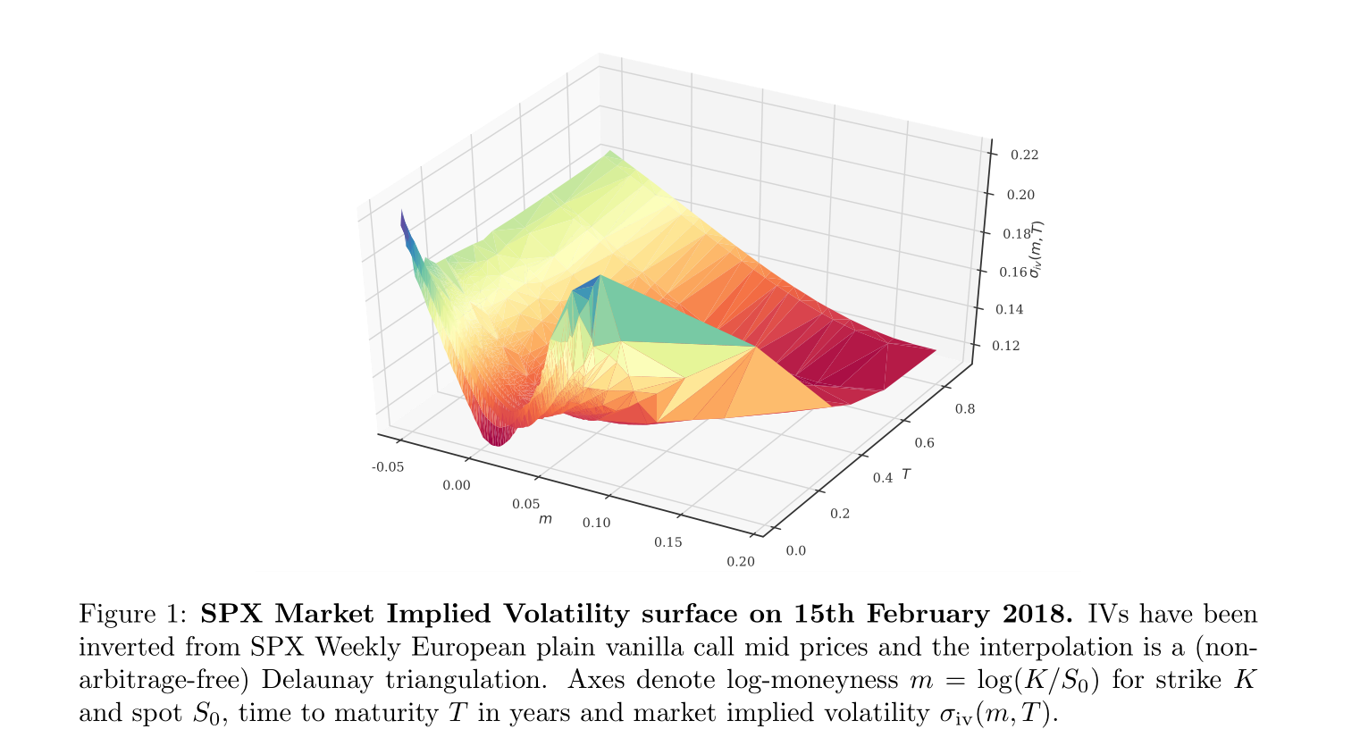
从隐含波动率按 moneyness 和 maturity 的变化可以观察到存在着著名的 smiles 和 at-the-money(ATM) skews 现象，与 BS 公式相悖．特别的，Bayer, Friz, and Gatheral 经验性地表明 ATM skew 符合如下形式：

$$\left|\frac{\partial }{\partial m}{\sigma }_{\mathrm{iv}}(m,T)\right|\sim T^{-0.4},T\to 0\text{\hspace{1em}(1)}$$ 其中 $m$ 为 $\log$ moneynessand ，$T$ 为 time to maturity .

根据 Gatheral ，扩散的随机波动率模型不能复现当 time to maturity 趋于零时 volatility skew 的幂指数爆炸现象，反而表现为常数现象．

RSV 可定义为一族连续路径的随机波动率模型，其瞬时波动率由一个 Holder 正则性比布兰运动小的随机过程驱动，通常刻画为 Hurst 系数 H<1/2 的分形布朗运动．

这种范式转变的证据现在是 overwhelming ，一方面在物理测度下，时间序列分析表明对数已实现波动率的 Holder 正则为 0.1 阶；另一方面，在定价测度下经验性观察也表明在零附近由模型能够生成 power-law behaviour 的 volatility skew．

模型的一大难点来自于分形布朗运动的非马尔科夫性．

本文介绍两种方法

• one-step approach : 直接学习从隐含波动率曲面到模型参数的映射，
• two-step approach : 第一步学习从模型参数到期权价格的映射，然后根据实际市场价格校准模型．又分为 point-wise approach 和 grid-wise approach，前者将行权价和到期日作为输入，后者事先设定好这两项．

二．模型校准概述（未使用神经网络）

校准（calibration）意思是调整模型参数以使得模型曲面符合由欧式期权通过BS公式计算出的经验隐含波动率曲面．

假设模型有一个参数集 $\Theta$ 决定， i.e.，由 $\theta \in \Theta$．进一步，我们假设期权由参数集 $\zeta \in Z$ 决定．E.g.，对看涨看跌期权我们有 $\zeta =(T,k)$，分别为到期日和 log-moneyness．有些参数由市场观测得到，如现价、利率等，不在校准过程中．定价映射为 $$(\theta ,\zeta )\mapsto P(\theta ,\zeta )$$ 带参数 $\theta$ 的模型中带参数 $\zeta$ 的期权的价格．我们通过 $\mathcal{P}(\zeta )$ 给定了有限子集 $\zeta \in Z^{\prime }\subset Z$ 以及所有可能的期权参数对应的期权价格．校准是决定模型参数以使模型价格 $(P(\theta ,\zeta ){)}_{\zeta \in Z^{\prime }}$ 和市场价格 $(\mathcal{P}(\zeta ){)}_{\zeta \in Z^{\prime }}$ 在给定距离度量下最小，i.e.: $$\hat{\theta }=\underset{\theta \in \Theta }{\mathrm{argmin}}\delta \left((P(\theta ,\zeta ){)}_{\zeta \in Z^{\prime }},(\mathcal{P}(\zeta ){)}_{\zeta \in Z^{\prime }}\right).$$

事实上，最常用的 $\delta$ 是加权最小二乘： $$\hat{\theta }=\underset{\theta \in \Theta }{\mathrm{argmin}}\sum _{\zeta \in Z^{\prime }}{w}_{\zeta }(P(\theta ,\zeta )-\mathcal{P}(\zeta ){)}^2$$ 这里的权重 $w_{\zeta }$ 反映了 $\zeta$ 对应期权的重要性以及 $\mathcal{P}(\zeta )$ 的可靠性．例如可以选择 bid-ask spread 的倒数．

只要模型参数比 $\left|Z^{\prime }\right|$ 少，此时就是超定(overdetermined)的非线性最小二乘问题，通常采用数值迭代的方法解决，如 Levenberg-Marquardt（LM）算法．

rBergomi ：表示为 ${\mathcal{M}}^{\text{rBergomi }}\left({\Theta }^{\text{rBergomi }}\right)$ ，参数 $\theta =\left({\xi }_0,\eta ,\rho ,H\right)\in {\Theta }^{\text{rBergomi }}$ ，例如可以设为 $${\Theta }^{\mathrm{rBergomi}}={\mathbb{R}}_{>0}\times {\mathbb{R}}_{>0}\times [-1,1]\times ]0,1/2[$$ 模型基于如下系统 $$\begin{array}{rl}d{X}_t& =-\frac{1}{2}{V}_{t}dt+\sqrt{V_t}d{W}_t,\text{ for }t>0,X_0=0\\ V_t& ={\xi }_0(t)\mathcal{E}\left(\sqrt{2H}\eta {\int }_0^t(t-s{)}^{H-1/2}d{Z}_s\right),\text{ for }t>0,V_0=v_0>0\end{array}$$ 其中 $H$ 是 Hurst 系数，$\eta >0$，$\mathcal{E}(\cdot )$ 是 Wick exponential，${\xi }_0(\cdot )>0$ 表示初始forward variance curve， $W$ 和 $Z$ 是以 $\rho \in [-1,1]$ 相关的布朗运动．

三．深度校准

3.1 one-step approach

Hernandez A. Model calibration with neural networks[J]. Available at SSRN 2812140, 2016.

直接学习校准过程，即将模型参数视作市场价格（隐含波动率）的函数，i.e. $${\Pi }^{-1}:(\mathcal{P}(\zeta ){)}_{\zeta \in Z^{\prime }}\mapsto \hat{\theta }$$ 更具体地，训练神经网络基于标签数据 $\left(x_i,y_i\right)，i=1，\dots ,N$， $$x_i=(\mathcal{P}(\zeta ){)}_{\zeta \in Z_i^{\prime }}$$ 及其对应标签 $$y_i={\hat{\theta }}_i$$

3.2 two-step approach

首先学习定价映射，将模型参数映射为市场价格（或隐含波动率），然后使用标准校准方法进行校准．我们用 $\tilde{P}(\theta ,\zeta )\approx P(\theta ,\zeta )$ 表示 $\tilde{P}$ 是 $P$ 的通过神经网络得到的近似．然后第二步我们进行校准 $$\hat{\theta }=\underset{\theta \in \Theta }{\mathrm{argmin}}\delta \left((\tilde{P}(\theta ,\zeta ){)}_{\zeta \in Z^{\prime }},(\mathcal{P}(\zeta ){)}_{\zeta \in Z^{\prime }}\right)\text{\hspace{1em}(2)}$$

两步方法相较而言最大的好处如下：

• 神经网络只负责期权定价，所以能用人工数据来训练．
• 自然地将误差分为定价误差和模型误差．神经网络表现和模型对市场适应性做出的调整相互独立．

3.2.1 two-step approach: 逐点训练（pointwise）和基于网格(grid-based)训练

In this section, we examine its advantages and present an analysis of the objective function with the goal to enhance learning performance. Within this framework, the pointwise approach has the ability to asses the quality of $\tilde{P}$ using Monte Carlo or PDE methods, and indeed it is superior training in terms of robustness.

Pointwise learning

step 1:学习映射 $\tilde{P}(\theta ,T,k)={\tilde{\sigma }}^{\mathcal{M}(\theta )}(T,k)$ 即上述（2）式令 $\zeta =(T,k)$．在标准化期权（vanilla option，$(\zeta =(T,k))$）情况下，我们可以直接学习隐含波动率映射 $\mathrm{map}{\tilde{\sigma }}^{\mathcal{M}(\theta )}(T,k)$，而不是期权定价的映射 $\tilde{P}(\theta ,T,k)$．用 $F(w;\theta ,\zeta )$ 表示神经网络，最优化问题如下： $$\hat{\omega }:=\underset{w\in {\mathbb{R}}^n}{\mathrm{argmin}}\sum _{i=1}^{N_{\text{Train }}}{\eta }_i{\left(\tilde{F}\left(w;{\theta }_i,T_i,k_i\right)-{\tilde{\sigma }}^{\mathcal{M}}\left({\theta }_i,T_i,k_i\right)\right)}^2$$

Step 2: 解决经典的模型校准步骤： $$\hat{\theta }:=\underset{\theta \in \Theta }{\mathrm{argmin}}\sum _{j=1}^m{\beta }_j{\left({\tilde{\sigma }}^{\mathcal{M}(\theta )}\left(\theta ,T_j,k_j\right)-{\sigma }_{\mathrm{BS}}^{\mathrm{MKT}}\left(k_j,T_j\right)\right)}^2$$

这里 $\tilde{P}(\theta ,T,k)$ 或者 ${\tilde{\sigma }}^{\mathcal{M}(\theta )}(T,k)$ 被替换成 step1 中的近似网络 $\tilde{F}(\hat{\omega };\theta ,T,k)$ ．

第一步中，关键在于训练数据和网络结构的选择．训练数据在于选择 $\theta$ 和 $\zeta$ $(=(T,k)$ 的‘先验’的、有实际意义的分布．

Implicit & grid-based learning

用 $\Delta :={\left\{k_i,T_j\right\}}_{i=1,j=1}^{n,}{m}_{i=1}$ 记关于到期日和行权价的网格．则

step 1：学习映射 $\tilde{F}(\theta )={\left\{{\sigma }_{BS}^{\mathcal{M}(\theta )}\left(T_i,k_j\right)\right\}}_{i=1,j=1}^{n,m}$，输入是 $\theta \in \Theta$，输出是 ${\left\{{\sigma }_{\mathrm{BS}}^{\mathcal{M}(\theta )}\left(T_i,k_j\right)\right\}}_{i=1,j=1}^{n,m}$ 这样的 $n\times m$ 网格．$\tilde{F}$ 取值在 ${\mathbb{R}}^L$ 中，其中 $L=$ strikes $\times$ maturities $=nm.$最优化问题变为如下： $$\hat{\omega }:=\underset{w\in {\mathbb{R}}^n}{\mathrm{argmin}}\sum _{i=1}^{N_{\text{Train }}^{\text{reduced }}}\sum _{j=1}^L{\eta }_j{\left(\tilde{F}{\left({\theta }_i\right)}_j-{\sigma }^{\mathcal{M}}\left({\theta }_i,T_j,k_j\right)\right)}^2$$ 其中 $N_{\text{Train }}=N_{\text{Train }}^{\text{reduced }}\times L$． Step 2: $$\hat{\theta }:=\underset{\theta \in \Theta }{\mathrm{argmin}}\sum _{i=1}^L{\beta }_j{\left(\tilde{F}(\theta {)}_i-{\sigma }_{\mathrm{BS}}^{\mathrm{MKT}}\left(T_i,k_i\right)\right)}^2$$

这里期权的参数 $\zeta =(T,k)$ 是固定了的，不再是学习的一部分．

3.2.2 pointwise versus grid-based

• 最大的不同在于 grid-based 在遇到不在网格上的 T,K 时需要手动插值
• grid-based 方法自然地有 reduction of variance ，
• pointwise 中对使样本符合实际金融数据的操作更简单，改变采样的分布．而 grid-wise 则是通过改变权重或者网格密度．
• grid-based 方法可以看做是一种降低维度的操作，将输入的维度转移到了输出的维度．

四．Pratical implementation

4.1 网络结构与训练

1. 隐藏层为 3 层的全连接前馈神经网络，每层 30 个结点
2. 输入维度记 $=n$
3. 输出维度为 $=11\times 8$
4. 总共有 $(n+1)\times 30+3\times (1+30)\times 30+(30+1)\times 88=30n+5548$ 个参数．
5. 激活函数选择 Elu， ${\sigma }_{\text{Elu }}=\alpha \left(e^x-1\right)$，梯度下降选择 Adam．

4.2 校准

使用第二节中讲的 LM 等算法．

五．数值实验

5.1定价近似网络的速度和精确度

※Deep learning volatility: a deep neural network perspective on pricing and calibration in (rough）volatility models※

Horvath B, Muguruza A, Tomas M. Deep learning volatility: a deep neural network perspective on pricing and calibration in (rough) volatility models[J]. Quantitative Finance, 2021, 21(1): 11-27.

Github 代码

fBm的 Monte-Carlo 模拟

1.理论基础

Horvath B, Jacquier A J, Muguruza A. Functional central limit theorems for rough volatility[J]. Available at SSRN 3078743, 2017.

Notations: 在单位区间 $\mathbb{I}:=[0,1]上,\mathcal{C}(\mathbb{I})$ 表示连续函数空间， ${\mathcal{C}}^{\alpha }(\mathbb{I})$ 表示 $\alpha$-Hölder 连续函数空间， $\alpha \in (0,1)$ ． ${\mathcal{C}}^1(\mathbb{I})$ 和 ${\mathcal{C}}_b^1(\mathbb{I})$ 是 $\mathbb{I}$ 上连续可微和有界连续可微函数空间．

1.1. Hölder spaces and fractional operators

For $\beta \in (0,1]$, the $\beta$-Hölder space ${\mathcal{C}}^{\beta }(\mathbb{I})$, with the norm $$\Vert f{\Vert }_{\beta }:=|f{|}_{\beta }+\Vert f{\Vert }_{\infty }=\underset{\genfrac{}{}{0ex}{}{t,s\in \mathbb{I}}{t\ne s}}{\sup }\frac{|f(t)-f(s)|}{|t-s{|}^{\beta }}+\underset{t\in \mathbb{I}}{\max }|f(t)|$$ is a non-separable Banach space. Following the spirit of Riemann-Liouville fractional operators recalled in Appendix $\mathrm{A}$, we introduce the class of Generalised Fractional Operators (GFO). For any $\lambda \in (0,1)$ we introduce the intervals $${\Re }^{\lambda }:=\{\alpha \in (-1,1)\text{ such that }\alpha +\lambda \in (0,1)\}$$ ${\Re }_{+}^{\lambda }:={\Re }^{\lambda }\cap (0,1),{\Re }_{-}^{\lambda }:={\Re }^{\lambda }\cap (-1,0)$, and the space ${\mathcal{L}}^{\alpha }:=\left\{u\mapsto u^{\alpha }L(u):L\in {\mathcal{C}}_b^1(\mathbb{I})\right\}$, for any $\alpha \in {\Re }^{\lambda }$

Definition 1.1. For any $\lambda \in (0,1)$ and $\alpha \in {\mathfrak{R}}^{\lambda }$, the GFO associated to $g\in {\mathcal{L}}^{\alpha }$ is defined on ${\mathcal{C}}^{\lambda }(\mathbb{I})$ as $$\left({\mathcal{G}}^{\alpha }f\right)(t):=\{\begin{array}{ll}{\int }_0^{t}f(s)\frac{\mathrm{d}}{\mathrm{d}t}g(t-s)\mathrm{d}s,& \text{ if }\alpha \in [0,1-\lambda )\\ \frac{\mathrm{d}}{\mathrm{d}t}{\int }_0^{t}f(s)g(t-s)\mathrm{d}s,& \text{ if }\alpha \in (-\lambda ,0)\end{array}\text{\hspace{1em}(1.1)}$$ We shall further use the notation $G(t):={\int }_0^{t}g(u)\mathrm{d}u$, for any $t\in \mathbb{I}$. Of particular interest in mathematical finance are the following kernels and operators: $$\begin{array}{lll}Riemann-Liouville:& g(u)=u^{\alpha },& for\alpha \in (-1,1)\\ Gammafractional:& g(u)=u^{\alpha }{\mathrm{e}}^{\beta u},& for\alpha \in (-1,1),\beta <0\\ Power-law:& g(u)=u^{\alpha }(1+u{)}^{\beta -\alpha },& for\alpha \in (-1,1),\beta <-1\end{array}\text{\hspace{1em}(1.2)}$$

Proposition 1.2. For any $\lambda \in (0,1)$ and $\alpha \in {\mathfrak{R}}^{\lambda }$, the operator ${\mathcal{G}}^{\alpha }:{\mathcal{C}}^{\lambda }(\mathbb{I})\to {\mathcal{C}}^{\lambda +\alpha }(\mathbb{I})$ is continuous.

We develop here an approximation scheme for the following system, generalising the concept of rough volatility in the context of mathematical finance, where the process $X$ represents the dynamics of the logarithm of a stock price process: $$\begin{array}{rlr}\mathrm{d}{X}_t& =-\frac{1}{2}{V}_t\mathrm{d}t+\sqrt{V_t}\mathrm{d}{B}_t,& X_0=0\\ V_t& =\Phi \left({\mathcal{G}}^{\alpha }Y\right)(t),& V_0>0\end{array}\text{\hspace{1em}(1.3)}$$ with $\alpha \in \left(-\frac{1}{2},\frac{1}{2}\right)$, and $Y$ the (strong) solution to the stochastic differential equation $(1.4)$ $$\mathrm{d}{Y}_t=b\left(Y_t\right)\mathrm{d}t+a\left(Y_t\right)\mathrm{d}{W}_t,Y_0\in {\mathcal{D}}_Y\text{\hspace{1em}(1.4)}$$

where ${\mathcal{D}}_Y$ denotes the state space of the process $Y$, usually $\mathbb{R}$ or ${\mathbb{R}}_{+}.$The two Brownian motions $B$ and $W$, defined on a common filtered probability space $\left(\Omega ,\mathcal{F},{\left({\mathcal{F}}_t\right)}_{t\in \mathbb{I}},\mathbb{P}\right)$, are correlated by the parameter $\rho \in [-1,1]$, and the functional $\Phi$ is assumed to be smooth on ${\mathcal{C}}^1(\mathbb{I}).$ This is enough to ensure that the first stochastic differential equation is well defined. It remains to formulate the precise definition for ${\mathcal{G}}^{\alpha }Y$ (Proposition 1.4) to fully specify the system (1.3) and clarify the existence of solutions. Existence and (strong) uniquess of a solution to the second $\mathrm{SDE}$ in (1.4) is guaranteed by the following standard assumption :

Assumption 1.3. There exist $C_b,C_a>0$ such that, for all $x,y\in {\mathcal{D}}_Y$ $$|b(x)-b(y)|\le C_b|x-y|\text{ and }|a(x)-a(y)|\le C_a\sqrt{|x-y|}$$

Proposition 1.4. For any $\alpha \in {\mathfrak{R}}^{1/2}$ ，the equality $\left({\mathcal{G}}^{\alpha }W\right)(t)={\int }_0^{t}g(t-s)\mathrm{d}{W}_s$ holds almost surely for $t\in \mathbb{I}$．

Example 1.5. This example is the rough Bergomi model introduced by Bayer, Friz and Gatheral, where $$V_t={\xi }_0(t)\mathcal{E}\left(2\nu C_H{\int }_0^t(t-s{)}^{\alpha }\mathrm{d}{W}_s\right)$$ with $V_0,\nu ,{\xi }_0(\cdot )>0,\alpha \in {\Re }^{1/2}$ and $\mathcal{E}(\cdot )$ is the Wick stochastic exponential. This corresponds exactly to $(1.3)$ with $g(u)\equiv u^{\alpha },Y=W$ and $$\Phi (\phi )(t):={\xi }_0(t)\exp \left(2\nu C_H\phi (t)\right)\exp \left\{-2{\nu }^2{C}_H^2{\int }_0^t(t-s{)}^{2\alpha }\mathrm{d}s\right\}$$

1.2 The approximation scheme

We now move on to the core of the project, namely an approximation scheme for the system (1.3). The basic ingredient to construct approximating sequences is a family of iid random variables, which satisfies the following assumption: Assumption 1.6. The family ${\left({\xi }_i\right)}_{i\ge 1}$ forms an iid sequence of centered random variables with finite moments of all orders and $\mathbb{E}\left[{\xi }_1^2\right]={\sigma }^2>0$

Following Donsker and Lamperti, we first define, for any $\omega \in \Omega ,n\ge 1,t\in \mathbb{I}$, the approximating sequence for the driving Brownian motion $B$ as $$B_n(t):=\frac{1}{\sigma \sqrt{n}}\sum _{k=1}^{\lfloor nt\rfloor }{\xi }_k+\frac{nt-\lfloor nt\rfloor }{\sigma \sqrt{n}}{\xi }_{\lfloor nt\rfloor +1}\text{\hspace{1em}(1.5)}$$ As will be explained later, a similar construction holds to approximate the process $Y$ : $$Y_n(t):=\frac{1}{n}\sum _{k=1}^{\lfloor nt\rfloor }b\left(Y_n^{k-1}\right)+\frac{nt-\lfloor nt\rfloor }{n}b\left(Y_n^{\lfloor nt\rfloor }\right)+\frac{1}{\sigma \sqrt{n}}\sum _{k=1}^{\lfloor nt\rfloor }a\left(Y_n^{k-1}\right){\zeta }_k+\frac{nt-\lfloor nt\rfloor }{\sigma \sqrt{n}}a\left(Y_n^{\lfloor nt\rfloor }\right)\zeta \lfloor nt\rfloor +1\text{\hspace{1em}(1.6)}$$ where $Y_n^k:=Y_n\left(t_k\right)$ and ${\mathcal{T}}_n:=\left\{t_k=\frac{k}{n}\right\}.$ Here $\{\xi {\}}_{i=1}^{\lfloor nt\rfloor }$ and $\{\zeta {\}}_{i=1}^{\lfloor nt\rfloor }$ satisfy Assumption $1.6$, with appropriate correlation structure between the pairs ${\left\{\left({\zeta }_i,{\xi }_i\right)\right\}}_{i=1}^{\lfloor nt\rfloor }$ that will be made precise later. We shall always use $\left({\xi }_i\right)$ to denote the sequence generating $B$ and $\left({\zeta }_i\right)$ the one generating $W$. Consequently, we deduce an approximating scheme (up to the interpolating term which decays to zero by Chebyshev's inequality) for $X$ as $$X_n(t):=-\frac{1}{2n}\sum _{k=1}^{\lfloor nt\rfloor }\Phi \left({\mathcal{G}}^{\alpha }{Y}_n\right)\left(t_k\right)+\frac{1}{\sigma \sqrt{n}}\sum _{k=1}^{\lfloor nt\rfloor }\sqrt{\Phi \left({\mathcal{G}}^{\alpha }{Y}_n\right)\left(t_k\right)}\left(B_n^{k+1}-B_n^k\right)\text{\hspace{1em}(1.7)}$$ All the approximations above, as well as all the convergence statements below should be understood pathwise, but we omit the $\omega$ dependence in the notations for clarity. The main result here is a convergence statement about the approximating sequence ${\left(X_n\right)}_{n\ge 1}$． As usual in weak convergence analysis, convergence is stated in the Skorokhod space $\left(\mathcal{D}(\mathbb{I}),\Vert \cdot {\Vert }_{\mathcal{D}}\right)$ of càdlàg processes equipped with the Skorokhod topology. Theorem 1.7. The sequence ${\left(X_n\right)}_{n\ge 1}$ converges weakly to $X$ in $\left(\mathcal{D}(\mathbb{I}),\Vert \cdot {\Vert }_{\mathcal{D}}\right)$. The construction of the proof allows to extend the convergence to the case where $Y$ is a $d$-dimensional diffusion without additional work. The proof of the theorem requires a certain number of steps: we start with the convergence of the approximation $\left(Y_n\right)$ in some Hölder space, which we translate, first into convergence of the stochastic integral in $(1.3)$, then, by continuity of the mapping $\Phi$, into convergence of the sequence $\left(\Phi \left({\mathcal{G}}^{\alpha }{Y}_n\right)\right)$. All these ingredients are detailed in Section 1.3 below. Once this is achieved, the proof of the theorem itself is relatively straightforward.

1.3. Monte-Carlo.

Theorem 1.7 introduces the theoretical foundations of Monte-Carlo methods (in particular for path-dependent options) for rough volatility models. In this section we give a general and easy-to-understand recipe to implement the class of rough volatility models (1.3). For the numerical recipe to be as general as possible, we shall consider the general time partition $\mathcal{T}:={\left\{t_i=\frac{iT}{n}\right\}}_{i=0,\dots ,n}$ on $[0,T]$ with $T>0$.

Algorithm 1.8 (Simulation of rough volatility models). (1) Simulate two $\mathcal{N}(0,1)$ matrices $$\begin{gathered} {\left\{{\xi }_{j,i}\right\}}_{j=1,\dots ,M} \\ i=1,\dots ,n \end{gathered}$$ and $$\begin{gathered} {\left\{{\zeta }_{j,i}\right\}}_{j=1,\dots ,M} \\ i=1,\dots ,n \end{gathered}$$ with $\mathrm{corr}\left({\xi }_{j,i},{\zeta }_{j,i}\right)=\rho$; (2) simulate M paths of $Y_n$ viad $$Y_n^j\left(t_i\right)=\frac{T}{n}\sum _{k=1}^{i}b\left(Y_n^j\left(t_{k-1}\right)\right)+\frac{T}{\sqrt{n}}\sum _{k=1}^{i}a\left(Y_n^j\left(t_{k-1}\right)\right){\zeta }_{j,k},i=1,\dots ,n\text{ and }j=1,\dots ,M$$ and also compute $$\Delta Y_n^j\left(t_i\right):=Y_n^j\left(t_i\right)-Y_n^j\left(t_{i-1}\right),i=1,\dots ,n\text{ and }j=1,\dots ,M$$ (3) Simulate $M$ paths of the fractional driving process ${\left(\left({\mathcal{G}}^{\alpha }{Y}_n\right)(t)\right)}_{t\in \mathcal{T}}$ using $${\left({\mathcal{G}}^{\alpha }{Y}_n\right)}^j\left(t_i\right):=\sum _{k=1}^{i}g\left(t_{i-k+1}\right)\Delta Y_n^j\left(t_k\right)=\sum _{k=1}^{i}g\left(t_k\right)\Delta Y_n^j\left(t_{i-k+1}\right),i=1,\dots ,n\text{ and }j=1,\dots ,M$$ The complexity of this step is in general of order $\mathcal{O}\left(n^2\right)$ (see Appendix $[\mathrm{B}$ for details). However, this step is easily implemented using discrete convolution with complexity $\mathcal{O}(n\log n)$ (see Algorithm [B.4 in Appendix $[\mathrm{B}$ for details in the implementation). With the vectors $\mathfrak{g}:={\left(g\left(t_i\right)\right)}_{i=1,\dots ,n}$ and $\Delta Y_n^j:=$ ${\left(\Delta Y_n^j\left(t_i\right)\right)}_{i=1,\dots ,n}$ for $j=1,\dots ,M$, we can write ${\left({\mathcal{G}}^{\alpha }{Y}_n\right)}^j(\mathcal{T})=\sqrt{\frac{T}{n}}\left(\mathfrak{g}\ast \Delta Y_n^j\right)$, for $j=1,\dots ,M$, where $\ast$ represents the discrete convolution operator. (4) Use the forward Euler scheme to simulate the log-stock process, for all $i=1,\dots ,n,j=1,\dots ,M$, as $$X^j\left(t_i\right)=X^j\left(t_{i-1}\right)-\frac{1}{2}\frac{T}{n}\sum _{k=1}^i\Phi {\left({\mathcal{G}}^{\alpha }{Y}_n\right)}^j\left(t_{k-1}\right)+\sqrt{\frac{T}{n}}\sum _{k=1}^i\sqrt{\Phi {\left({\mathcal{G}}^{\alpha }{Y}_n\right)}^j\left(t_{k-1}\right)}{\xi }_{j,k}$$

Remark:

• When $Y=W$, we may skip step (2) and replace $\Delta Y_n^j\left(t_i\right)$ by $\sqrt{T/n}{\zeta }_{i,j}$ on step (33).
• Step (3) may be replaced by the Hybrid scheme algorithm 11 only when $Y=W$.

Antithetic variates in Algorithm 1.8 are easy to implement as it suffices to consider the uncorrelated random vectors ${\zeta }_j:=\left({\zeta }_{j,1},{\zeta }_{j,2},\dots ,{\zeta }_{j,n}\right)$ and ${\xi }_j:=\left({\xi }_{j,1},{\xi }_{j,2},\dots ,{\xi }_{j,n}\right)$, for $j=1,\dots ,M.$ Then $\left(\rho {\xi }_j+\bar{\rho }{\zeta }_j,{\xi }_j\right),(\rho {\xi }_j-$ $\bar{\rho }{\zeta }_j,{\xi }_j),\left(-\rho {\xi }_j-\bar{\rho }{\zeta }_j,-{\xi }_j\right)$ and $\left(-\rho {\xi }_j+\bar{\rho }{\zeta }_j,-{\xi }_j\right)$, for $j=1,\dots ,M$, constitute the antithetic variates, which significantly improves the performance of the Algorithm 1.8 by reducing memory requirements, reducing variance and accelerating execution by exploiting symmetry of the antithetic random variables.

1.3.1 Enhancing performance. A standard practice in Monte-Carlo simulation is to match moments of the approximating sequence with the target process. In particular, when the process is Gaussian, matching first and second moments suffices. We only illustrate this approximation for Brownian motion: the left-point approximation may be modified to match moments as $$\left({\mathcal{G}}^{\alpha }W\right)\left(t_i\right)\approx \frac{1}{\sigma \sqrt{n}}\sum _{k=1}^{i}g\left(t_k^{\ast }\right){\zeta }_k,\text{ for }i=0,\dots ,n\text{\hspace{1em}(1.8)}$$ where $t_k^{\ast }$ is chosen optimally. Since the kernel $g(\cdot )$ is deterministic, there is no confusion with the Stratonovich stochastic integral, and the resulting approximation will always converge to the Itô integral. The first two moments of ${\mathcal{G}}^{\alpha }W$ read $$\mathbb{E}\left(\left({\mathcal{G}}^{\alpha }W\right)(t)\right)=0\text{ and }\mathbb{V}\left(\left({\mathcal{G}}^{\alpha }W\right)(t)\right)={\int }_0^{t}g(t-s{)}^2\mathrm{d}s$$ The first moment of the approximating sequence 1.8 is always zero, and the second moment reads $$\mathbb{V}\left(\frac{1}{\sigma \sqrt{n}}\sum _{k=1}^{j-1}g\left(t_k^{\ast }\right){\zeta }_k\right)=\frac{1}{n}\sum _{k=1}^{j-1}g{\left(t_k^{\ast }\right)}^2$$ Equating the theoretical and approximating quantities we obtain $\frac{1}{n}g{\left(t_k^{\ast }\right)}^2\mathrm{d}s={\int }_{t_{k-1}}^{t_k}g(t-s{)}^2\mathrm{d}s$ for $k=1,\dots ,n$, so that the optimal evaluation point can be computed as $$g\left(t_k^{\ast }\right)=\sqrt{n{\int }_{t_{k-1}}^{t_k}g(t-s{)}^2\mathrm{d}s},\text{ for any }k=1,\dots ,n$$ In the Riemann-Liouville fractional Brownian motion case, $g(u)=u^{H-1/2}$, and the optimal point can be computed in closed form as $$t_k^{\ast }={\left(\frac{n}{2H}\left[{\left(t-t_{k-1}\right)}^{2H}-{\left(t-t_k\right)}^{2H}\right]\right)}^{1/(2H-1)},\text{ for each }k=1,\dots ,n$$

1.3.2 Reducing Variance.

As Bayer, Friz and Gatheral, a major drawback in simulating rough volatility models is the very high variance of the estimators, so that a large number of simulations are needed to produce a decent price estimate. Nevertheless, the rDonsker scheme admits a very simple conditional expectation technique which reduces both memory requirements and variance while also admitting antithetic variates. This approach is best suited for calibrating European type options. We consider ${\mathcal{F}}_t^B=\sigma \left(B_s:s\le t\right)$ and ${\mathcal{F}}_t^W=\sigma \left(W_s:s\le t\right)$ the natural filtrations generated by the Brownian motions $B$ and $W.$ In particular the conditional variance process $V_t\mid {\mathcal{F}}_t^W$ is deterministic. As discussed by Romano and Touzi, and recently adapted to the rBergomi case by McCrickerd and Pakkanen, we can decompose the stock price process as $${\mathrm{e}}^{X_t}=\mathcal{E}\left(\rho {\int }_0^t\sqrt{\Phi \left({\mathcal{G}}^{\alpha }Y\right)(s)}\mathrm{d}{B}_s\right)\mathcal{E}\left(\sqrt{1-{\rho }^2}{\int }_0^t\sqrt{\Phi \left({\mathcal{G}}^{\alpha }Y\right)(s)}\mathrm{d}{B}_s^{\perp }\right):={\mathrm{e}}^{X_t^1}{\mathrm{e}}^{X_t^2}$$ and notice that $$X_t\mid \left({\mathcal{F}}_t^W\wedge {\mathcal{F}}_0^B\right)\sim \mathcal{N}\left(X_t^1-\left(1-{\rho }^2\right){\int }_0^t\Phi \left({\mathcal{G}}^{\alpha }Y\right)(s)\mathrm{d}s,\left(1-{\rho }^2\right){\int }_0^t\Phi \left({\mathcal{G}}^{\alpha }Y\right)(s)\mathrm{d}s\right)$$ Thus $\exp \left(X_t\right)$ becomes log-normal and the Black-Scholes closed-form formulae are valid here (European, Barrier options, maximum,...). The advantage of this approach is that the orthogonal Brownian motion $B^{\perp }$ is completely unnecessary for the simulation, hence the generation of random numbers is reduced to a half, yielding proportional memory saving. Not only this, but also this simple trick reduces the variance of the Monte-Carlo estimate, hence fewer simulations are needed to obtain the same precision. We present a simple algorithm to implement the rDonsker with conditional expectation and assuming that $Y=W$.

Algorithm 1.9 (Simulation of rough volatility models with Brownian drivers). Consider the equidistant grid $\mathcal{T}$. (1) Draw a random matrix ${\left\{{\zeta }_{j,i}\right\}}_{j=1,\dots ,M/2}$ with unit variance, and create antithetic variates ${\left\{-{\zeta }_{j,i}\right\}}_{j=1,\dots ,M/2}$; (2) Create a correlated matrix $\left\{{\xi }_{j,i}\right\}$ as above; (3) Simulate $M$ paths of the fractional driving process ${\mathcal{G}}^{\alpha }W$ using discrete convolution: $${\left({\mathcal{G}}^{\alpha }W\right)}^j(\mathcal{T})=\sqrt{\frac{T}{n}}\left(\mathfrak{g}\ast {\zeta }_j\right),j=1,\dots ,M$$ and store in memory $\left(1-{\rho }^2\right){\int }_0^T{\left({\mathcal{G}}^{\alpha }W\right)}^j(s)\mathrm{d}s\approx \left(1-{\rho }^2\right)\frac{T}{n}{\sum }_{k=0}^{n-1}{\left({\mathcal{G}}^{\alpha }W\right)}^j\left(t_k\right)=:{\Sigma }^j$ for each $j=1,\dots ,M$ (4) use the forward Euler scheme to simulate the log-stock process, for each $i=1,\dots ,n,j=1,\dots ,M$, as $$X^j\left(t_i\right)=X^j\left(t_{i-1}\right)-\frac{{\rho }^2}{2}\frac{T}{n}\sum _{k=1}^i\Phi {\left({\mathcal{G}}^{\alpha }W\right)}^j\left(t_{k-1}\right)+\rho \sqrt{\frac{T}{n}}\sum _{k=1}^i\sqrt{\Phi {\left({\mathcal{G}}^{\alpha }W\right)}^j\left(t_{k-1}\right)}{\xi }_{j,i}$$ (5) Finally, we have $X^j(T)\sim \mathcal{N}\left(X_T^j-{\Sigma }^j,{\Sigma }^j\right)$ for $j=1,\dots ,M;$ we may compute any option using the Black-Scholes formula. For instance a Call option with strike $K$ would be given by $C^j(K)=$ $\exp \left(X_T^j\right)\mathcal{N}\left(d_1^j\right)-K\mathcal{N}\left(d_2^j\right)$ for $j=1,\dots ,M$, where $d_1^j:=\frac{1}{\sqrt{{\Sigma }^j}}\left(X_T^j-\log (K)+\frac{1}{2}{\Sigma }^j\right)$ and $d_2^j=d_1^j-\sqrt{{\Sigma }^j}$ Thus, the output of the model would be $C(K)=\frac{1}{M}{\sum }_{k=1}^M{C}^j(K)$